• Leverage Jupyter Notebook for Reporting on your BIM360/ACC Environment

    Leverage Jupyter Notebook for Reporting on your BIM360/ACC Environment

    Introduction

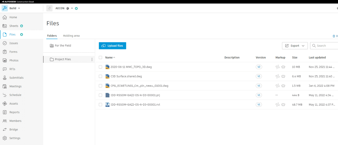
    Autodesk Construction Cloud (ACC) (see Figure 1) is a cloud-based application that allows design teams to manage their drawings and building models in a centralized way.  ACC has a well-defined Restful (REST) API interface that makes it easy to extract and report on all manner of operational information.  Using Python, Jupyter Notebook, and some ubiquitous Python libraries it is quite simple to create a customizable dashboard that can be leveraged on-demand by BIM Managers and IT Admins alike.

    Figure 1 – Autodesk Construction Cloud 


    What do you need?

    So what do we need to know in order to get started?  To prepare you will need access to Autodesk Construction Cloud, which I won’t cover here, and of course a Forge account that will allow you to setup and connect an application to your ACC hub.  You can find more information on setting up a forge application in this link.  Secondly, you will need to install Anaconda which is a powerful Python based data science platform that allows users to easily install and run a wide variety of Python libraries.  Once you install Anaconda, you will need to install a few libraries including the following:

    • requests –allows users to make HTTP calls to cloud services;
    • json – allows users to serialize the resulting Json to easily access attributes;
    • matplotlib – allows users to create rich data visualizations such as graphs (Matlab);
    • pandas – provides users with several useful data management tools; and
    • datetime plus dateutil – which allows us to easily perform date functions such as time zone conversion.

    You can find more information on installing Anaconda at this link.

    Finally, you will need to create a new Anaconda environment (see link) and install the libraries listed above along with Jupyter Notebook.  Jupyter Notebook can be installed from the Anaconda prompt with the following:

    (env) PS C:\user> conda install jupyter notebook

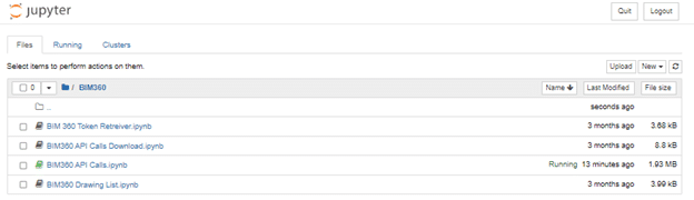
    Once Jupyter Notebook is installed you can simply type jupyter notebook at the command prompt and hit enter to open the console in a new browser window or tab. (see Figure 2)

    Figure 2 – Jupyter Notebook Starting Page

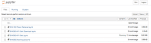
    The starting page provides access to all the notebooks in your development environment.

    One more thing before you get started, you will need to set up an application in Autodesk Forge.  You will then attach that application to your ACC instance so you can access the information through the REST API.  More instructions on setting this up can be found by following this link.

    Creating a Dashboard

    A dashboard is intended to be a simple graphical data-driven interface that provides a window into operational activities and events.  The dashboard must be two things

    1. simple to understand; and
    2. relevant

    Some thought should be given to what you want to report on but some examples are

    • drawing type distribution statistics which provide some insight into software usage; and
    • user role distribution statistics which provide insight into who is doing what.

    Once you have determined what you are going to report on, you can then start building your notebook.

    Building and Organizing Your Notebook

    Jupyter Notebook allows users to structure their code into cells which provides a way to step through your code.  This is very important for debugging as you can easily isolate sections of code which provides better code management.

    You can start by importing all relevant Python libraries. (see Figure 3)

    Figure 3 – Import Python libraries to extend the functionality of the core Python environment


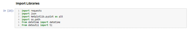
    Once the correct libraries are imported to the Jupyter Notebook session you can start setting up the appropriate properties starting with the authorization call. (see Figure 4)

    Figure 4 – Parameters to be used for collecting authorization token

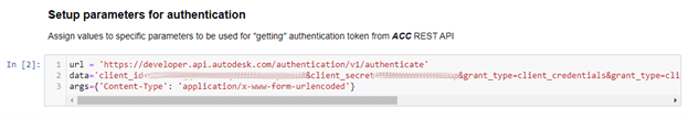
    These parameters are then used in an HTTP call using the request library to return the appropriate authorization token.  Note: you must set up the correct scope(s) to ensure the permissions you have when the REST API is called are adequate.  Some example scopes are as follows:

    • data:read
    • data:write
    • data:create

    However, there are many others, which you can find out more about by visiting this link.

    Collecting the Data

    Now you can collect the appropriate data for your dashboard.  To do this you will need to find the correct REST Endpoints.  Some of the endpoints used for this demonstration are:

    Using these endpoints, you can simply leverage the request Python library functions to retrieve the data

    • users = requests.get(url, data=data, headers=auth)

    The json Python library can be used to serialize the resulting “user” object for easy access to the data attributes.

    • json = json.loads(users.text)

    Now you can iterate through the json object and populate python lists to create a “data table” object.  Those data table objects can then be simply plugged into any number of data visualization objects such as a pandas dataframe or a Matlab graph.

    Visualizing the Dashboard

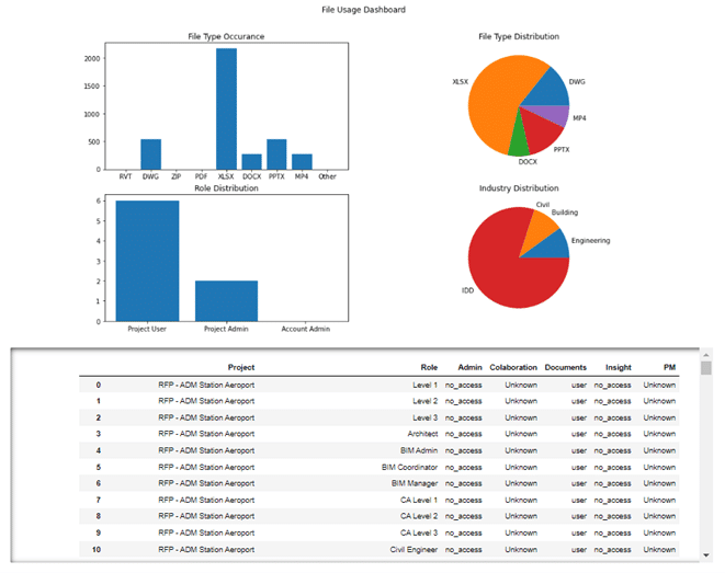
    So now you have the data to visualize, how do you get it into a dashboard?  Now you can leverage the final Python library of this demo, matlibplot.  This library allows users to plug the lists of data created above into several different graphical representations.  Figure 5 illustrates a set of graphic plots created with matlibplot (Matlab) as well as a data table produced from a pandas data frame.  You can see that these graphical data objects can be organized into a meaningful dashboard that can be reused and even shared with others in your organization.

    Figure 5 – Jupyter Notebook Dashboard with Data Frame Table

    Development and Sharing

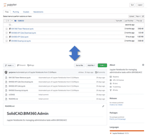
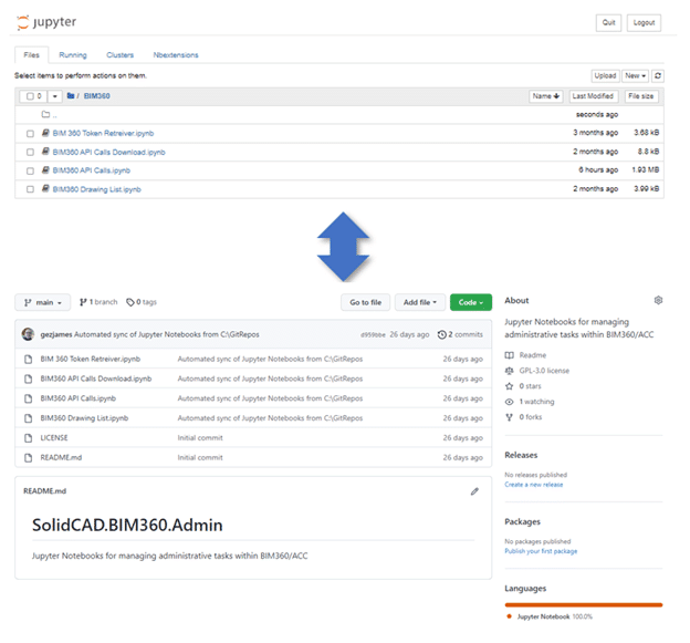
    A brief word on sharing these dashboards throughout the organization and for tracking development of the notebooks.  It is very simple to publish these notebooks to a GitHub repository (see Figure 6) that will allow other users to access the notebooks as permitted.  GitHub can also track versions of the different notebooks to make it possible to go back in time to find previous code which makes it easier to do code trials.  You can also create different code branches that allow multiple developers to work on the notebooks simultaneously.

    To do this you will need to create a GitHub repository, load your notebooks to that repository and then clone the repository to your local machine.   Once you have the notebooks in a local repository, you can set the custom location for your notebooks to that repo by accessing the configuration file, typically located at C:\Users\<username>\.jupyter\jupyter_notebook_config.py and then updating the line that starts c.NotebookApp.notebook_dir = by adding the location of your notebook repo to the end.  This will ensure the start page shows your development repository.

    Figure 6 – Committing Jupyter Notebooks to GitHub

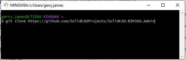
    There are a few ways that you can synchronize your notebook location to GitHub.  Of course, you can do it manually but accessing the repository from the web interface, or you can install GitBash (see Figure 7) for windows and perform the repository functions by command line or batch file.

    Figure 7 – GitBash for Windows

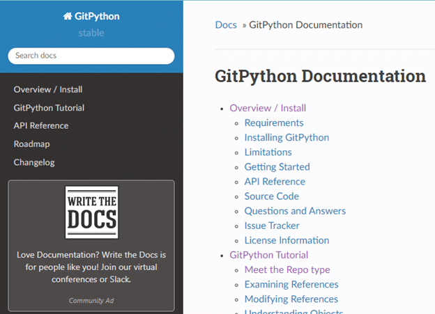
    Finally, you can create your own utility to do the synchronization in a more directed way.  There are a variety of Python libraries such as PyGithub or GitPython that can help create your own Jupyter Notebook to synchronize your notebooks with GitHub. (see Figure 8)

    Figure 8 – GitPython Python Library for working with GitHub

    Other Use Cases

    While the use of Jupyter Notebook and Python as tools to generate meaningful reports, there are many other uses that could be investigated.  I personally work with many clients to develop ETL (extract, transform, load) strategies to bring mission-critical data into their hosted and cloud environments.  Part of this process almost always requires some Python coding to perform tasks the OOB (out of the box) software cannot do.  I find Jupyter Notebook an extremely powerful IDE for doing code development, allowing me to perform debugging and quality control activities without a lot of software knowledge.  Additionally, Python can be used to access other cloud-based platforms with a REST API such as Fusion 360 Manage which is Autodesk’s primary PLM (product lifecycle management) platform.  Jupyter Notebook could be a way to report on content in this platform as well as extend the functionality to ensure implementations of these frameworks are successful.

    Conclusion

    BIM and IT managers are tasked with ensuring the efficient flow of data through their organizations’ design and engineering processes.  This requires easy access to any number of information products including usage, data, and role statistics.  Python can easily be accessed through the Jupyter Notebook interface and, in conjunction with the ACC REST API, provides a very useful tool for any BIM or IT manager to report on these items.

    The scripts can be created to be very flexible and easily shared, allowing users to pass their own information into the process and create rich dashboards for business and engineering analytics.  The ACC and BIM 360 APIs are very well documented so anyone with a bit of understanding of REST and Python can get started creating these products.  Together, these are very flexible and powerful frameworks for collecting data from cloud services and for reporting on current environmental conditions.

    Civil 3D: Profile Grade Intersections

    The goal in this example is to design the profile where each grade is an even number.  It’s not as obvious as you might think.  Thanks to my colleagues Dave Hill and Jae Kwon for pointing out the proper tool.

    Read on to learn more…

    Begin by modelling the first 2 segments.  I’ll assume you know the best tools for this, but I’ll give you a hint.  Use the Grid View; it’s your friend here.


    To model the last 5% grade is not entirely obvious.  Yes, a 5% tangent can be drawn from the end of the 1% grade, but it doesn’t end in the right place.

    We sort of want to draw backwards from the end of the red profile and then extend the 1% grade.

    Use this tool and follow the prompts.  First select the 1% grade, then pick Station and Elevation and the tie-in point.  Then enter the grade, in this case -5% (the grade from the intersected PVI).


    C’est voilà.


    Civil 3D: Model Existing Underground Utilities Efficiently

    Civil 3D: Model Existing Underground Utilities Efficiently

    Must you draw existing gas, tel, and other similar underground utilities for your projects?  If you’re not using the technique described below, you’re using too much time!  Read on to find out more.

    Join us at Infrastructure University, session 3, on October 20th for more information about this technique. For now:

    Facts:

    1. For nearly every civil engineering project, we must identify existing features on our construction drawings so they may not be disturbed during construction and so we may design proposed works without conflicting with these existing features. They must appear in both plan and profile.
    2. It can take considerable time to draw and label them in the plan, and even more project them into profile.
    3. When there is an edit to the alignment, the profile locations must be recalculated, taking more time.
    4. Experiments have shown that it can take 84 seconds to draw each utility. Then 26 more seconds each when the alignment is edited.
    5. Using the technique described below, the time is reduced from 84 seconds to 20 seconds. But 0 seconds when the alignment is edited.
    6. For 160 utilities:
      1. 3.7 hours using the manual technique.                   69 minutes each time the alignment is edited.
      2. 53 minutes using the automated technique.         No extra time when the alignment is edited.

    Method

    1. Create pressure network parts lists, one for each utility. Assign styles accordingly.
    2. Create pressure networks, one for each utility. Assign the parts list and label styles accordingly.
    3. Model the existing utilities as pressure networks and project them into profile. The depth below ground can be automated.

    CTC Licensing Model Change – What you need to know!


    With the release of the 23.0.0 version of all the CTC Software tools, CTC has taken the opportunity to update its licensing model.

    Licensing for any of the CTC suites of tools was broken up into tiers of licensing with maintenance attached or differences depending on how many employees were in the company. It was tedious to explain, and not too efficient to implement.

    Starting with the 23.0.0 release of the suites, CTC is moving to a CSL model of licensing. This Cloud Shared Licensing is much more in line with the SaS model of software delivery. However, this is deliberately not the named user licensing that Autodesk has moved to. The CSL model is intended to simplify access to the tools while maintaining the flexibility of the network licensing style of license.

    Put simply, the CSL model is a cloud-hosted version of the network licensing most of us are familiar with. This means there is no need for installing license managers on local servers, all users need is internet access to use the CTC tools. The CSL is hosted on the new CTC website that was launched in conjunction with the 23.0.0 suite releases.

    With the new website, there have been additional efficiencies added by automating tasks like the option to renew automatically and automatic fulfilment of orders. The new website will also give administrators detailed insight into their teams’ suite usage and the ability to control the allocation of licenses with the creation of Groups of users on the website.

    The move to CSL was done for efficiency for everyone. It simplifies and standardizes access to the tools, allows for instant license allocation, offers to report on the usage of suites and tools, and simplifies pricing models.

    One thing to note is that the 2022 and older versions of the CTC Suites still only work with the legacy licensing and cannot use the CSL model.


    Want to learn about this licensing in more detail? Visit: View Recording (gotowebinar.com).

     If you have questions regarding this new licensing model for the CTC Software, your SolidCAD Account Manager will be more than happy to help!


    How to Create Intelligent Custom Labels with Expressions in Civil 3D

    Introduction

     Figure 1 – Dynamically Labelled Basement Elevations

    Today we see how we can make labelling much easier and consistently accurate in Civil 3D. “Expressions” are used to create user properties that can automate a lot of label text generation and positioning as well. The expression techniques used here are useful for every kind of custom Civil 3D labels. There are several labelling methods:

    1. Manual text
    2. Dynamic block (with attributes)
    3. Civil 3D Labels (with Expressions)

    To set up the easiest labelling workflow, Civil 3D labels with expressions is usually the way to go. We spend a bit of time setting things up, but once it’s setup, it takes little time to do the labelling and even less time to update any changes. Dynamic blocks with attributes and parameters can be just as good, but we’ll save that discussion for another time.

    Sample Use Case

    In this example, we just want to input the finished floor elevation, how far down the other elevations are, and what lot number we are labelling. We want the label to take care of the rest, including calculations and label positioning.

    It can be done for either profile views or section views. A sample DWG is available for download so that you can see exactly how everything was set up. For now, we will go over some high-level notes on what was done.

    Profile View Implementation

    • The finished floor is represented by a TIN surface. The TIN surface is simply defined by a rectangle breakline that’s at the finished floor elevation.
    • The actual label is done as a “Lines” label of the FF surface profile, on a profile view.
    • To set up a label style properly, we first need some expressions setup- BsmtFlrOffset (-2.9): how many meters down from FF the basement floor is
    • BsmtFlr ({Tangent Start Elevation}+BsmtFlrOffset): calculated basement floor elevation
    • BtmFtgOffset (-3.25): how many meters down from FF the bottom of footing is

    BtmFtg ({Tangent Start Elevation}+BtmFtgOffset): calculated bottom of footing elevation

    • ViewScale (2): The viewscale of the profile view. 1:500 = 1000/500 = 2.
    • PVExaggeration (10): Vertical exaggeration of the profile view.
    • LabelPosition1 (BsmtFlrOffset*ViewScale*PVExaggeration/1000): Y offset used to position the basement floor label. It takes into account the view scale (1:500) and the vertical exaggeration (x10).
    • LabelPosition2 (BtmFtgOffset*ViewScale*PVExaggeration/1000): Y offset used to position the bottom of footing label.
    • LabelPositionLot (LabelPosition1/2): Y offset used to position the lot number label. Half way in between FF label and the basement floor label.

    Sample drawing has four label components:

    • FF elevation label: use the “Tangent Start Elevation” property, attached to the feature.
    • Basement floor elevation label: uses expression BsmtFlr, positioned by expression LabelPosition1 for its Y offset.
    • Bottom of Footing elevation label: uses expression BtmFtg, positioned by expression LabelPosition1 for its Y offset.
    • Lot number text label: Since the profile is named with the lot name (LOT 81). Positioned by expression LabelPositionLot for its Y offset.

    It takes some initial setup, but once that’s done, all it takes is just applying a Lines label in the profile view and that’s it! Elevations and label positions are automatically calculated and positioned. The only adjustments that might have to be made is editing some expressions to note what elevation offsets, view scale, and exaggeration are used.

    Section View Implementation

    The implementation is essentially the same as the profile, with a few differences.

    • Major Offset label type is used
    • Sections actually have “Drawing Scale Conversion” property available out of the box. If the scale is 1:200, “Drawing Scale Conversion” property is 1/200 = 0.005. This makes section labels automatically position correctly for all scales unlike the profile ones!

    Conclusion

    Civil 3D label expressions can help us set up all sorts of custom labelling that automates calculations as well as label positioning.

    It takes a little bit of investment to get used to, but once you set up one or two, it becomes fairly easy and can greatly expand the capabilities of your template. That in turn, helps everyone not only save time, but be more consistent, as dynamic labels help us avoid forgetting label updates as designs change. Navisworks has the ability to open various file types. It can also read embedded data if the proper object enabler is installed. Fortunately, Autodesk has one specifically for Plant 3D. You can download the 2021 version here.

    Here’s an example of a Plant 3D model in Navisworks without an object enabler. You can see that some shapes aren’t displayed properly, and it is not reading the embedded data.

    Here is the same Plant 3D model with the object enabler installed. All the components are displayed correctly, and the embedded data is being displayed in the properties section.

    With the Plant 3D model in Navisworks, the file can now be saved as an NWD file and delivered to external parties. All they need is Navisworks Freedom to view the file, which can be downloaded for free from Autodesk.  This is one of many features available in Navisworks. Apart from a robust 3D viewer it can perform tasks such as clash detection and animation.

    If you would like to learn more, Navisworks training is available as a supplementary course to SolidCAD’s Plant 3D course curriculum. Please email us at contact training@solidcad.ca.

    In the next blog, we will look at how to utilize the Navisworks plug in within Plant 3D. Stay tuned!


    Autodesk Desktop Connector Update

    Autodesk Desktop Connector 

    Autodesk regularly updates the Desktop Connector with fixes to defects and some basic functionality updates; this update is no different, but there is one major feature update which has been on users’ wish lists for a while.

    Users can now change the location of the Workspace to another fixed drive location. This will be very welcome to many IT departments. Formerly, the Desktop Connector would only save to the user’s local C Drive. Many users’ C Drives are not large enough to accommodate the added load of storing files locally when using the Autodesk Construction Cloud. IT can install larger file drives onto users’ computers since the Desktop Connector can now store files on a drive other than C. 

    Click here to see the documentation and to download it.

    Enjoy!


    Civil 3D Assemblies: Tool Palette or Block Library?

    Civil 3D Assemblies: Tool Palette or Block Library?

    Civil 3D comes shipped with pre-configured assemblies that may or nay not fit your needs.  We created another BLOG post here to show how to create your own and share them with others in your team.  There is another way…read on.

    The Cole’s notes are:

    • Make a new drawing.
    • Create your assembly in this new drawing placed at 0,0.
    • Insert that drawing into your design and explode the resulting block.

    In the linked article above, we suggested creating a tool palette.  This works well for blocks so they may be placed on the correct layers.  For assemblies, since this block will be exploded, this is not a requirement.  Might there be an easier way?  There is.  You see, tool palettes require a little maintenance.  The trick below does not.

    AutoCAD’s Block Library

    In Civil 3D 2022 or later, open the new block palette introduced in version 2020.  The option I’m about to illustrate is not available with 2020 or 2021.  You will see two things: a Library tab (red) and a button to select a folder (blue).  Clicking the folder button will prompt you to select a folder containing drawings.  If each of those drawings is an individual assembly, your job is done.  Drag and drop one of those into your drawing and ensure it is exploded.  You’ve just inserted an assembly.

    No maintenance is required.  Just save a new drawing with a new assembly into that folder and the next time AutoCAD is started, you’ll see the new content.  If you prefer to have all assembly blocks defined in a single drawing, that’s fine too, simply right click the drawing and choose…

    Enjoy!

    Recap: 2023 Release

    Recap: 2023 Release

    Autodesk has just released their Point Cloud management application, Recap 2023.  Click here to join the live webinar on April 19thClick here for Autodesk documentation.  Read on to find out more.

    Here is the new feature:

    Autodesk Docs

    Store point clouds in Autodesk Docs and share them with stakeholders.  The Autodesk Viewer has been enhanced to allow Point Clouds to be viewed, measured, and annotated within an internet browser.

    Infraworks: 2023 Release

    Infraworks: 2023 Release

    Autodesk has just released its Civil visualization and analysis application, Infraworks 2023.  Click here to join the live webinar on April 19thClick here for Autodesk documentation.  Read on to find out more.

    Here are some of the new features:

    Parametric Content

    Easily check for updated content from the styles palette.

    The Infrastructure Parts Editor plugin for Inventor is no longer required, point to any Inventor Part or Assembly, and it will be added as a new style.

    Structural Bridge Design

    Bi-directional workflow between structural analysis and the parametric bridge model has been enabled.

    Command Search

    Use simple terms to search for the commands you need when you need them. And, this tool keeps a history of your past actions, making it even simpler.

    Cloud Credits

    Cloud credits are no longer required for Watershed Analysis and Profile Optimization.

    Civil 3D: 2023 Release

    Civil 3D: 2023 Release

    Autodesk has just released its flagship Civil Engineering modelling application, Civil 3D 2023.  Click here to join the live webinar on April 19thClick here for Autodesk documentation.  Click here for the 2023 help page.

    Read on to find out more.

    There are several useful new features, but I know the question on almost everyone’s mind is “Has the format changed?”  The answer, happily, is no!  2018 is still the native format for drawings saved with AutoCAD and Civil 3D 2023.  Backwards compatibility has been maintained.

    In no particular order, check out some of the new features and enhancements:

    2022.1 Update

    All the features from the 2022.1 updates are included in 2023.

    Performance

    Significant performance enhancements are reported.

    Grading Optimization

    • Help Center – get assistance in the form of tutorials, sample files, and workflows.
    • Progress Bar – see visual cues about the progress.
    • It’s available for download now!

    Project Explorer

    • Display custom notes and quantities.
    • It’s available for download now!

    Geotechnical Modeler

    • It’s available for download now!

    Pressure Networks

    • Keyword Search – search for parts to model.
    • Property Sets – show in profile view labels.
    • Profile Editing – reduce PVIs and other enhancements.
    • Cut Length – specify a cut length if none is defined in the catalogue.

    Rail

    • CANT – label enhancements.
    • Catalogue – replace a catalogue when modified.

    Additional Updates

    • Corridor Targets – target multiple surfaces, dynamic target layers.
    • Property Sets – dynamically updates with changes to the corridor.